C1 - Control Theory Applications Assignment

Aims

• To illustrate how control theory is applied to a real design problem. The example used is for a conveyor system used to position parts in a manufacturing cell.
• To demonstrate how modern computer-aided design (CAD) software can be used to simplify the design process.

Digital Platform and Software

This Control Laboratory C1 will be online based using Zoom and the software MATLAB/Simulink will be used during the session. The Zoom link will be sent through an announcement in Week 9. The Matlab Online version will be used, and this is accessible at: https://uk.mathworks.com/products/matlab-online.html Please sign in or create a new account through the above link using your university’s email address at the start of the session. Alternatively, you can also use any downloaded version of MATLAB if installed.

Introduction

One common application of control systems theory is the design of position servos. These are mechanisms giving either rotational or translational motion, driven by a motor (electric, hydraulic or pneumatic) and equipped with a controller (usually electronic or microprocessor-based). Such systems are used in various applications, from lens auto-focus mechanisms in modern cameras to positioning mechanisms in computer-controlled machinery.

Figure 1 gives the schematic diagram for a conveyor system used to position parts in a manufacturing cell.

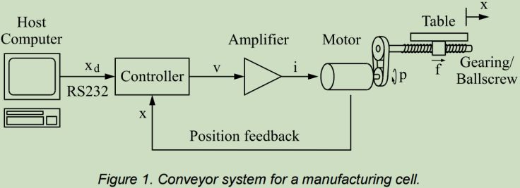
The purpose of the conveyor control system is to move a linear table, driven by an electric motor, to desired positions entered from a host computer.

The conveyor system is controlled by a controller which accepts commands from a host computer via an RS232 serial communications link. The controller also has interfaces for a number of transducers, and one of these is used to monitor the actual position of the table via a position transducer mounted on the motor (i.e., position feedback). The controller allows the user to program a control law that is suitable for the given application. Unfortunately, it is sometimes difficult to determine the best control law by trial and error since trying an unsuitable control law might cause damage to the system through excessive accelerations and motor loadings. Consequently, control theory is often used to model the system first, ascertain the system’s response to typical inputs and hence predict a suitable control law BEFORE the actual system is powered up.

The process of modelling the system is described below.

System Modelling

Consider each component of the system in turn.

Controller

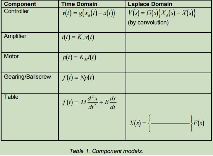
The controller accepts as inputs the desired table position Xd(t) and the actual table position x(t) obtained from a transducer mounted on the motor. The two values are compared and the error is fed to the control law which will for now be represented by some general functiong() . The resulting control action v(t) (a voltage) is given by:

v(t)=g(Xd(t)-x(t))

Amplifier

The amplifier is a high-power switched-mode current amplifier designed especially for driving DC servo motors. Although the amplifier itself contains a series of feedback loops, its overall characteristics can be accurately modelled by a linear relationship, so the current output i(t) is:

I(t)=kav(t)
Where ka is amplifier gain unit(units A/V)

Motor

The motor is a high-quality DC servo motor. It is explicitly designed to be powerful for its size and to have low rotor inertia (which means it can start and stop very quickly). The torque p(t) generated by the motor is proportional to the armature current, i.e.:

P(t)=Kmi(t)
Here, km is tearmed the motor torque constant( unit Nm/A )

Gearing/Ballscrew

The gearing and ballscrew transmit the torque generated by the motor to the table. The resulting force f (t) acting on the table is given by:

F(t)=Md^x/dt^2
where M is the mass of the table (units kg).

As the velocity of the table increases, frictional forces acting on the bearings of the motor, the gearing and the ballscrew will arise. These forces will tend to oppose the motion of the table, giving rise to the modified equation:

F(t)= Md^2x/dt^2+Bdx/dt
where B is a friction coefficient (units Ns/ m ).

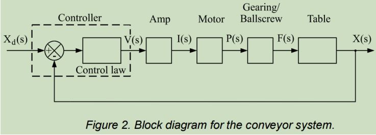
Having modelled each system component, the various models (equations 1-6) can be used to form a block diagram. However, equations (1) to (6) must be converted to the Laplace domain first.

Exercise - Transfer Functions and Block Diagrams

1. Convert the equations in Table 1 to the Laplace domain, assuming that all initial conditions are zero. Hence complete Table 1.
2. Use these equations to complete the block diagram shown in Figure 2.
3. Combine the same equations to generate a transfer function for the whole system. The transfer function for the whole system is:

X(s)/Xd(s)=

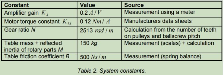
Having determined a block diagram and transfer function for the system, the only further parameters required to complete the system model are values for the system constants KA , K M , N, M and B. Table 2 gives values obtained through measurement or from manufacturers’ data sheets.

Simulation

The system model can now be used to try different control laws G(s)Determining the behaviour of the system under a particular control law involves choosing a typical input to the control system, applying this to the model and calculating the response.

Typical Inputs

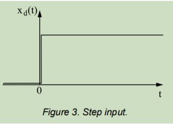
The input most commonly used to test position servo mechanisms is the step illustrated in Figure 3. The step is used as it highlights both transient and steady state responses.

Candidate Control Laws

A useful control law commonly used in position servo mechanisms is the proportional (P) control.

The P controller is simply a gain, i.eG(s) = KPwhere KP is a constant termed the proportional or position gain.

The P controller generates a control action proportional to the error signal. When applied to the conveyor, this generates a force that moves the table in a direction that reduces the difference between the desired and actual table positions. To investigate the effect of the P controller on the conveyor system, a computer simulation package called MATLAB/Simulink will be used.

MATLAB/Simulink

MATLAB/Simulink is a computer simulation package that was initially designed to perform matrix algebra but has now been extended through a series of toolboxes to perform a variety of different tasks. In particular, a “toolbox” called Simulink allows users to construct control system block diagrams and then analyse them graphically.

Exercise - Using MATLAB/Simulink

Use the MATLAB/Simulink to create a block diagram for the conveyor system and then determine the response to a step input of magnitude 0.02 m.

1. Run MATLAB and type simulink. This brings up a window named Simulink. (Be patient, when you do this for the first time, it may take a couple of minutes for the MATLAB window to appear).
2. From the Simulink window, select the Blank Model and a new window should appear, named “untitled”.
3. Open the Commonly Used Block tree from the Simulink library browser window by clicking the Simulink node and choosing the Commonly Used Block This library contains most of the elements required to construct the block diagram.
4. To start the block diagram, drag a gain element from the library window across to the new window. Double-click on it and use the dialog box to change the gain to 0.2 ( KA ). This will form the amplifier element in the block diagram.
5. Similarly, drag the gain elements across to form the motor and gearing elements.
6. Drag a sum element across to form the comparator. Double-click on it and set the signs to +- instead of ++.
7. Choose the Continuous node from the Simulink tree. Drag a transfer function (Transfer Fcn) element across to form the table element of the block diagram. Double-click on it and set the denominator coefficients to [150 500 0].
8. Drag a PID Controller element across to form the control law block. Doubleclick on it and set the proportional gain to 250 ( KP ) and both the derivative and integral gains to 0 ( K D and KI).
9. Connect the various blocks together by drawing in the links with the mouse pointer.
10. Choose Sources node from Simulink tree and drag across Step Input Double click on it and set the step time to 2, the initial value to 0 (default), the final value to 0.02, and the sample time to 0.001. Connect it to the input of the control system.
11. Open the Sinks block library and drag across a Scope Connect this to the output of the control system.
12. Save your Simulink model by clicking save or save as in your model window.
13. Set the stop time to 10 seconds (default).
14. Run the simulation by clicking the Run icon