Convergence Analysis and Grid Adaptation

Problem Description 

The purpose of this assignment is to develop a finite-volume solver to solve the equation 

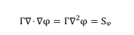
Where ? = ?(x, y) in ?, where ? is a rectangular domain of size Lx × Ly, ? is a constant  coefficient (used to describe a permeability, e.g. thermal conductivity), and ? is some arbitrary  scalar function (e.g. temperature). A similar term appears in the momentum equation of the  Navier-Stokes equations, as underlined in Eq. (2)

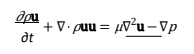
Thus, this assignment will be a first step towards developing a Navier-Stokes solver. In order to
discretize Eq. (1), a finite-volume approach is used which breaks up the domain ? into discrete
control volumes. Fig. 1 shows an example of the discretized domain for this assignment.

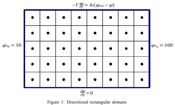
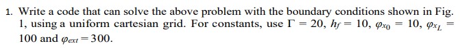
The boundary conditions in Fig. 1 are Dirichlet (fixed) at the x boundaries, a zero-gradient (insulated) boundary condition is applied at the bottom, while at the top there is a convective heat  flux boundary, which is typically used when two different materials are in contact (note that we  sometimes refer to this boundary as a Robin or mixed boundary condition and it is essentially a  linear combination of a Dirichlet and Neumann condition). For the convective heat flux boundary, the transfer coefficient hf and the external temperature ?ext are both fixed. 

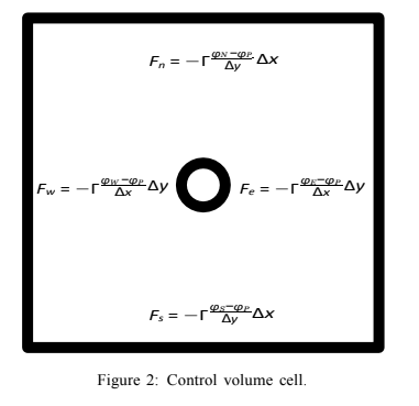
In order to discretize Eq. (1), consider a single control volume shown in Fig. 2. For a steady state case, the sum of the fluxes through the cell faces must be zero. The fluxes in Fig. 2 for each face are calculated using a simple centered finite-difference at each face (note: you should be able to come up with these fluxes yourself, it is an important exercise). Note that the sign convention is suchthat outgoing fluxes are considered positive.

Thus, solving Eq. (1) using the finite-volume method is really a matter of solving the following
equation:

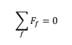
for each cell in Fig. 1, where f denotes a cell face. Note that the computation of the flux depends on
whether or not the face is an interior face (e.g. between two cells), or a boundary face. At
boundaries, the flux may be simple enough to compute directly, while for interior faces the solution
will depend on the solution of neighboring cells. To start, make sure you understand how to
compute the fluxes for each type of face. For boundary faces, it is fine to simply use a
backwards/forwards finite-difference to approximate the gradient (it can be shown that this is the
same as mirroring the cell across the boundary and applying a centered finite-difference across the
face, and shouldn’t affect the global accuracy of the solution). The most efficient way to solve this
problem is to assemble all the equations for each cell defined by Eq. (3) into a single linear
system of the form

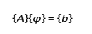
and solve it using your matrix solver from the previous assignment. This can be done using either
an iterative or direct solver.

Requirements

The requirements for this assignment are as follows:

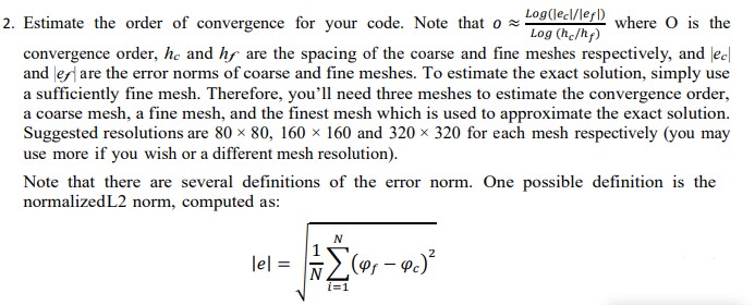
where N is the number of cells in the domain. Other definitions of the norm can also work.
The process for estimating order of convergence is as follows:

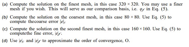
The main challenge in calculation of the order of convergence is that the coarse and the fine
meshes do not coincide with each other. So one needs to perform interpolation on the coarse
and the fine meshes to find the value of ”phi” at coincident points . To make this calculation
easier, one can also make use of scipy.interpolate.interp2d class:

This class allows you to approximate the results on the coarse and the fine meshes with
functions that use spline (e.g. linear, bi-cubic/bi-linear) interpolation, so you can find ”phi”
at any desired(x, y).

As shown in the example below, a function is created to interpolate “phi” on a mesh, where here x and
y store the coordinates of the mesh nodes and “phi” is a 2D array of the solution:

f = interpolate.interp2d(x, y, phi, kind=’cubic’)

This function can be called to find phi at any given (X0, Y0) on the mesh by interpolating your solution:

Phi_0 = f(X_0, Y_0)

3. Once your code is working for a uniform grid, allow the node spacing to vary. For example,
gradientsare often higher near boundaries, so it makes sense to accumulate more nodes there.
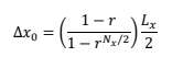
So, we may wish to apply “inflation”. First, we define an inflation factor r > 1. Then, we
computeour initial spacing by:

and each subsequent spacing is computed via:

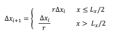
Note that you may need to re-scale your domain slightly to ensure the dimensions haven’t
changed. The procedure for applying inflation in the y direction is the same. Repeat the order
of convergence test from step 2, and comment on the results.

Are you struggling to keep up with the demands of your academic journey? Don't worry, we've got your back! Exam Question Bank is your trusted partner in achieving academic excellence for all kind of technical and non-technical subjects. Our comprehensive range of academic services is designed to cater to students at every level. Whether you're a high school student, a college undergraduate, or pursuing advanced studies, we have the expertise and resources to support you.

To connect with expert and ask your query click here Exam Question Bank