SEB113 Statistics: Correlation and Regression Assignment
- Subject Code :
SEB113
- Country :
Australia
Question 1: Linear Correlation
(a) An investigation is conduced into whether students' performances in reading are related to their performance in mathematics. Marks for reading and mathematics exams for eight students are shown in the table below.
| Student | 1 | 2 | 3 | 4 | 5 | 6 | 7 | 8 |
| Reading mark (x) | 59 | 68 | 64 | 83 | 75 | 63 | 81 | 73 |
| Maths mark (y) | 62 | 75 | 60 | 78 | 81 | 67 | 78 | 75 |
The linear correlation coefficient of this data is r=0.847.Assess whether the researchers could claim, with 95% confidence, that slope of the 'best-fit' straight line is different from zero, by answering the following questions.
- State the null and proposed hypothesis.
Proposed Hypothesis: The slope of the maths mark against the reading mark is not zero.
Null Hypothesis: The slope of the maths mark against the reading mark is 0. - State an appropriate statistical test and calculate an appropriate test statistic.
The test statistic is equal to the linear correlation coefficient between the maths mark and the reading mark. From question r = 0.847.
- Using the value of the test statistic from (ii) make a decision on the hypothesis test.
Critical value is shown using rCRIT.
The number of tails is 2.
The significance level is 0.05.
The sample size is 8.
rCRIT = r2,0.05,8 = 0.707 (from Table on page 7 of Exam Resource Sheet)
0.847 > 0.707 (r> rCRIT), therefore we accept the proposed hypothesis and conclude that the slope of the maths mark against the reading mark is not 0 and there is a correlation between these variables.
(b) An investigation is conducted into the relationship between the weight (g) and length (cm) of a species of fish. Measurements of seven fish at the same age are shown in the table below.
| Fish | 1 | 2 | 3 | 4 | 5 | 6 | 7 |
| Weight (x) | 142 | 190 | 240 | 263 | 330 | 350 | 400 |
| Length (y) | 23.0 | 27.3 | 24.9 | 30.0 | 27.5 | 28.6 | 25.6 |
The linear correlation coefficient of this data is r=0.393. Assess whether the researchers could claim, with 95% confidence, that slope of the 'best-fit' straight line is greater than zero, by answering the following questions.
- State the null and proposed hypothesis.
Proposed Hypothesis: The slope of the length against the weight of fish is greater than zero.
Null Hypothesis: The slope of the length against the weight of fish is zero. - State an appropriate statistical test and calculate an appropriate test statistic.
The test statistic is equal to the linear correlation coefficient between the fishs length and weight. From question r = 0.393.
- Using the value of the test statistic from (ii) make a decision on the hypothesis test.
Critical value is shown using rCRIT.
The number of tails is 1.
The significance level is 0.05.
The sample size is 7.
rCRIT = r1,0.05,8 = 0.669 (from Table on page 7 of Exam Resource Sheet)
0.393 < 0>
(c) *** An investigation was conducted into the relationship between temperature (?) and power consumption (kWh). Measurements are recorded at nine different locations and shown in the table below.
| Location | 1 | 2 | 3 | 4 | 5 | 6 | 7 | 8 | 9 |
| Temperature (x) | 20.1 | 22.2 | 23.4 | 24.1 | 25.1 | 26.1 | 26.4 | 27.1 | 27.2 |
| Power consumption (y) | 32000 | 33000 | 31000 | 32000 | 34000 | 33000 | 33000 | 36000 | 35000 |
The linear correlation coefficient of this data is r=0.681. Assess whether the researchers could claim, with 95% confidence, that slope of the 'best-fit' straight line is different from zero, by answering the following questions.
- State the null and proposed hypothesis.
- State an appropriate statistical test and calculate an appropriate test statistic.
- Using the value of the test statistic from (ii) make a decision on the hypothesis test.
Question 2: Statistics of Correlation and Regression
(a) In Question 3 from Practical Worksheet 3 we used Wolfram Alpha to plot the data and determine a 'best-fit' straight line for the data. Here we will use R.
- Make a new folder on your computer and name this SEB113R. You may have already created this folder in Week 5.
- Download " W10DataQ2a.xlsx" from Canvas and save this to your SEB113R folder.
- Open RStudio.
- Open a new R file, by clicking File -> New File -> R Script.
- Save the file, by clicking File -> Save As -> W10Question2a, to your SEB113R folder.
- Import the data, click File -> Import Dataset -> From Excel. Choose the "W10Question2a.xlsx" file and click Import.
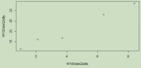
- Enter the following command into the R file (top left panel) and click Run, to plot the data plot(W10DataQ2a$x, W10DataQ2a$y)
- Enter the following command into the R file (top left panel) and click Run, to calculate the linear correlation, cor(W10DataQ2a$x, W10DataQ2a$y)
The linear correlation is r = 0.986.
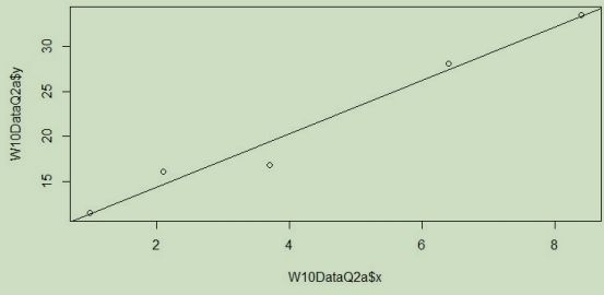
- Enter the following command into the R file (top left panel) and click Run, to determine an equation for best-fit straight line, lm(W10DataQ2a$y ~ W10DataQ2a$x, W10DataQ2a)
 Therefore, the equation for the line is:
 - Using the R output, state the slope and the y-intercept.
The slope is 2.970 and the y-intercept is 8.371
- Enter the following command into the R file (top left panel) and click Run, to plot the data with the bestfit straight line, abline(lm(W10DataQ2a$y ~ W10DataQ2a$x))
(b) *** In Week 5 you generated a file called "23se1surveydatatop50.xlsx". This file contained fifty randomly selected rows of results from the Statistics Portfolio Survey. If you have not yet generated this file there is a stepby-step instructional video on how to create this file on the SEB113 Canvas Week 5 Module. We will now explore this data set using linear correlation and regression.
- Choose two Quantitative - Continuous variables in the data set to analyse, for example "Foot" and "Height". A full list of variables in the Statistics Portfolio Survey results, and their descriptions, is appended to this document. If you are unsure whether your choices of variables are appropriate, ask your tutor in your workshop.
- State a question that you can explore with linear correlation and regression. If you are unsure whether your question is appropriate, ask your tutor in your workshop.
- Using R, plot your data.
- Using R, calculate the linear correlation coefficient.
- Using R, plot your data with the 'best-fit' straight line.
Hint: Question 2(a) is similar.
Question 3: Uncertainty in Linear Calibration
(a) An experiment is performed to measure the absorbance, The measurements are shown in the table. The equation for the straight line that best fits through the data of absorbance, A against concentration,C, is given by A=0.1224C-1.1760.
| Concentration, C | 22.5 | 25.0 | 27.5 | 30.0 |
| Absorbance, | 1.63 | 1.94 | 2.01 | 2.59 |
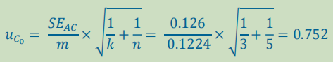
- Calculate the 95% confidence interval of the concentration,Co.
CI: C0 t2,?, n -2 x
CI: 205.686 t2,0.05, 5 - 2
x 0.752
t2,0.05, 3 = 3.18 (from Table on page 5 of Exam Resource Sheet)
CI: 205.686 3.18 x 0.752
CI: 205.686 2.39
205.686 - 2.39 = 203.296
205.686 + 2.39 = 208.076
203.296 ? C0 ? 208.076 - Building on Question 2(a), we now explore how to calculate residuals, the standard error of regression, and explore curvature in residuals.
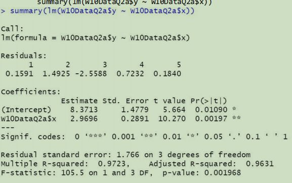
- Enter the following command into the R file (top left panel) and click Run, to calculate the residuals at each point. summary(lm(W10DataQ2a$y ~ W10DataQ2a$x))
The Residuals are 0.1591, 1.4925, -2.5588, 0.7232, and 0.1840.
- Enter the following command into the R file (top left panel) and click Run, to calculate the standard error of regression. SSRESID <- sum(resid(lm(W10DataQ2a$y ~ W10DataQ2a$x))^2) sqrt(SSRESID/(length(W10DataQ2a$x)-2)) Note: This uses the formula
The standard error of regression is 1.766.
- Enter the following command into the R file (top left panel) and click Run, to plot the residuals. plot(resid(lm(W10DataQ2a$y ~ W10DataQ2a$x)))
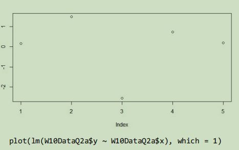
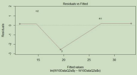
- Is there curvature in the residuals? What should a researcher do if they observe curvature (or systematic variation) in the plot of residuals?
It appears that the residuals do not have systematic variation. If a researcher were to observe systemic variation in the curvature, they should investigate the reason for the curvature occurring, whether it is due to error or a different model being required.
