Array-Based Binary Search Tree Implementation and Operations

Binary Trees

So far, every data structure we have looked at has been linear.  From arrays to linked lists, performance has depended on the the algorithms that support the structure.  For example, the Binary Search is able to eliminate half a sorted data set each time a comparison is made.  Now let’s look at a non-linear structure that has this binary feature built in.

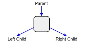
This chapter will introduce a tree structure that arranges data like the roots or branches of a tree.  This allows an algorithm that traverses it to divide the available data, much like the Binary Search does in an flat array.  The building block for a tree is a node, similar to the node in a linked list, but instead of being linked to the next node in a list, each node has “children” to the left and right below it.  The node is itself a child of a “parent” node above it.

More complex trees may have nodes with additional children, but for this course we will stick with just two per node, making it a Binary Tree.

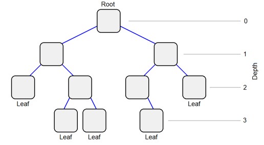
A binary tree has a single node at the top, or level 0, called the Root. Pairs of nodes are connected beneath the root to make additional levels. Each level can have twice as many nodes as the one above it. Nodes without any children are called leaves.

Yes, I know it’s upside down! Nearly every representation of a binary tree looks like this.

The depth of the tree is the lowest level, or the maximum distance from the root node. The tree on the previous page has a depth of 3. If all the nodes were populated at level 3, it would have 8 nodes. In general, the maximum number of nodes in a fully populated tree is:

1 + 2 + 4 + 8 + … + 2depth = 2(depth+1)-1

So a tree with a depth of 9 could have up to 1023 nodes. To get to any node, a function starts at the root, then moves left or right down the tree. In this imagined tree, it would only take 9 iterations to get to any element in the structure.

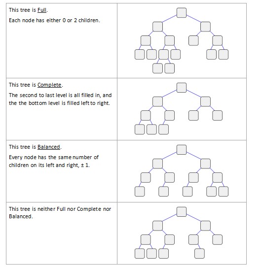
There are special terms used to describe how populated a tree is:

Binary Search Tree

It is necessary to have rules that determine if a node will be located to the left or right of an existing node.  This allows a value to be inserted into the structure, and then later retrieved without having to search the entire tree.  A Binary Search Tree (BST) is a specialization of the tree structure with rules described in this diagram:

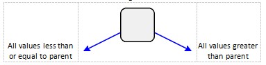
This will order the nodes in the tree so that smaller values go to the left, and larger values to the right.  A simple < or> operator can be used in the implementation.  Below are two tree examples:

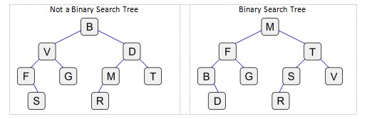
The tree on the left isn’t in any specific order.  If you wanted to find a value, you would have to check every node in the tree.  The tree on the left uses the BST rules, so you can find a value by starting at the root and working your way down.

So using the BST on the right, let’s say you wanted to find the letter D:

• Start at M
• D is less than M, so go left
• D is less than F, so go left
• D is greater than B, so go right
• D is found

And if you wanted to find the letter U:

• Start at M
• U is greater than M, so go right
• U is greater than T, so go right
• U is less than V so go left
• No node with U exists

If your search runs off the bottom of the tree, then you know the value isn’t there.  For a reasonably balanced tree, this search has O(Log₂N) operations.

Find & Insert

To insert a node into a tree, we have to find the appropriate place in the tree.  First, check the root.  If there is no root, then just put the node there and you’re done.  Otherwise, we need to move down the tree to an available location.  We’ll use a variable p to represent the new node, and q to represent the node in the tree.  A loop will compare p to q and either move left or right.  Once it gets to the correct spot (and empty location) attach the node there.

Insert BST - Empty Root

• Attach p as the root

Insert BST - Root Exists

• Set q = root
• Loop while p ?q
  • If p’s value <= q’s value

If q has no left child, attach p as q’s left child

Set q = q’s left child

• Otherwise

If q has no right child, attach p as q’s right child

Set q = q’s right child

The loop continues as long as p and q are not referring to the same node.  This can also be implemented as a function that returns immediately after p is attached.  Below is a picture illustrating the path a node will travel to it’s destination.

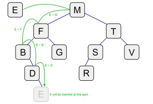
A function to just find a value would use the same algorithm above, but omit the steps that attach a new node.  The function could return true/false, or the location of the node.  We will see an implementation later on. 

If we have N random values to insert, this will take about O(NLog₂N) operations.  But if all the values are in ascending or descending order, the tree will be lopsided, with each node having a single child.  This would take O(N²) operations, because it is essentially appending to a linked list.  Later we will look at how to balance a tree for better performance.

Traversals

So how do we display this structure?  If we use the tree diagram, a data set with more than a few levels is going to take a lot of space (imagine taping sheets of paper together) or teeny-tiny print on the screen.  Instead, let’s look at algorithms that traverse the tree to create a linear list for output.

A traversal of a binary tree has to explore different branches, which is a non-linear process.  This task is an ideal candidate for a recursive solution.  A binary tree has three commonly used traversals.  Each has three parts:  output current node, explore left, and explore right.  The order these steps are done will determine the order of the entire ouput.

The most commonly used traversal is Left-Middle-Right.  The algorithm looks like this:

Function LMR

• If there is a left child, call LMR to process that child
• Output the current node
• If there is a right child, call LMR to process that child

This starts at the root, displays everything on the left side of the tree, then the root, then everything on the right side.  The same rules are used for the left and right sides.  This is also called an in-order traversal.  If the tree is a BST, then the output will be in ascending order.

LMR Animation

To output the tree in the reverse order, Right-Middle-Left, swap the processing of the left and right children:

Function RML

• If there is a right child, call RML to process that child
• Output the current node
• If there is a left child, call RML to process that child

This is called a reverse in-order traversal and will display a BST in descending order.

RML Animation

The LMR and RLM are the most frequently used traversals.  A pre-order (MLR) outputs the current node first, then the two children.  A post-order (LRM) outputs the children, then the current node.  There are also reverse versions of pre- and post- orders.

Size

We can use the same recursive steps as a traversal to count the number of nodes in the tree.  Instead of displaying the values, the count is increased.  Start by counting the current node, then add the count of the left children and then the right children.

Function Size

• count = 1
• If there is a left child, call Size for left child and add to count
• If there is a right child, call Size for right child and add to count
• Return count

Each node returns the number of nodes in its sub-tree.  Calling this function from the root will return the total nodes in the entire tree.  Every node has to be checked, so this is a O(N) operation.

Depth

Calculating the depth is a little trickier, because instead of just counting the nodes, we need to select which child has the deeper sub-tree.  Save the depth for the left and right sides, and return the larger.

Function Depth

• If there is a left child, L = Depth for left child
• If there is a right child, R = Depth for right child
• Return 1 + max(L,R)

We have to add 1 to count the current level, so that as the function recurses down the tree, the depth increases.  This will give us an almost correct value, since it assumes that the root is at level 1.  So to get the actual depth, call this function from the root, then subtract one.

If your tree is implemented with a container class, you will need two functions.  The first will start at the root and call the second recursive depth_r() function.  Any of the tree functions that require recursion will work this way.  One function to check the root, and a private recursive function to do the work.

Tree Container

• insert()
• find()
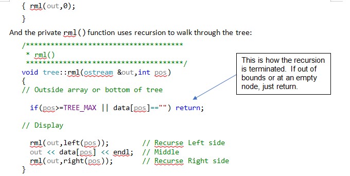
• output() rml()
• size() size_r()
• depth() depth_r()
• remove()

Array Implementation

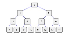
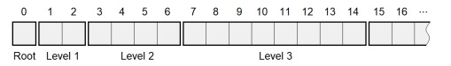
One way to store a binary tree is with an array.  The root goes at index 0 and its children at 1, 2. Their children go at 3, 4 and 5, 6.  The next row is indices 7-14, and so on:

If the tree is densely populated, then the array is a compact way to store it. If it isn’t, then the used elements will be spread out through the array. Here is the array mapping for the BST on the previous page:

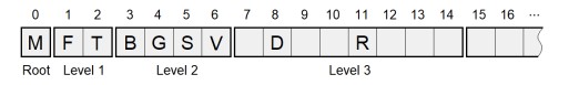
No extra storage is needed for pointers, because all the links between nodes and their children are built into the indices. We can calculate the index of a node’s children by doubling its index position to get to the next level, then adding 1 for the left child, or 2 for the right child.

Left = Position*2+1

Right = Position*2+2

We can also move back up the tree with the parent formula:

Parent = (Position-1)/2

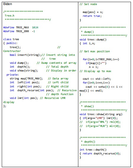
Remember the index is an integer, so division by two drops the remainder. These formulas can be implemented as inline functions:

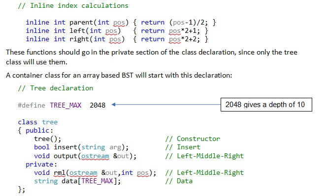
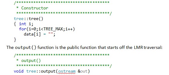
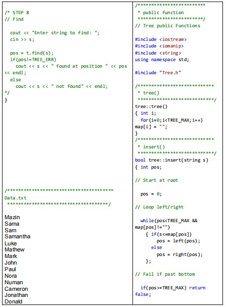
Other functions can be added as needed. The constructor has a linear loop that initializes all the strings to be empty.

The insert() function doesn’t use recursion. It starts at the root and walks down through the tree to an open node. The path is determined by comparing the argument to the data node and recalculating the index position.

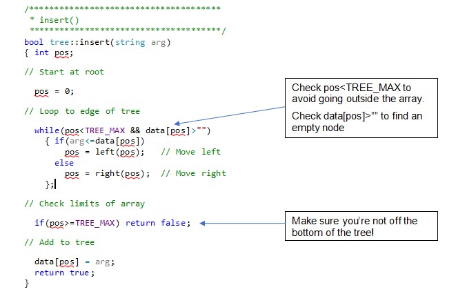
By updating pos, the index doubles and moves down a level each time around the loop. This is a O(Log2N) function. If pos lands on an open element, the argument is copied there.

Other functions can be implemented using the left() and right() functions to calculate indices of children nodes. They will either use a single loop to walk down the tree, or recursion to visit every node. That code isn’t given here. You will understand them better if by working on them in a lab assignment.

The find() function is very similar to the insert. Start at the root, and work left/right down the tree to find a match. If the pos index exceeds the length of the array or hits an empty element, then the argument isn’t in the tree. It should remind you of the Binary Search, where each time around the loop it is checked for a match, then one half of the data is selected.

Other functions like size() or depth() use recursive traversals similar to the output() and rml() pair. The size() function starts at 0 and calls size_r(). The depth() function starts at 0, calls depth_r() and subtracts 1 (see the previous discussion of Depth).

This implementation doesn’t have a remove() function. It’s possible, but very messy. Removing a node means having to adjust all the children below it. Let’s save that method for a version with pointers.

Recursion and binary tree.

Print a copy of your code files along with the outputs from steps 5, 7, and 9.

1- The notes of the binary tree are attached in D2L. The table below shows the following,

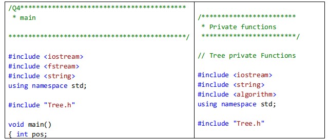
copy paste the code and data files shown in the table below,

Main.cpp, Tree.h, Tree Public.cpp, Tree Private.cpp, Data.txt

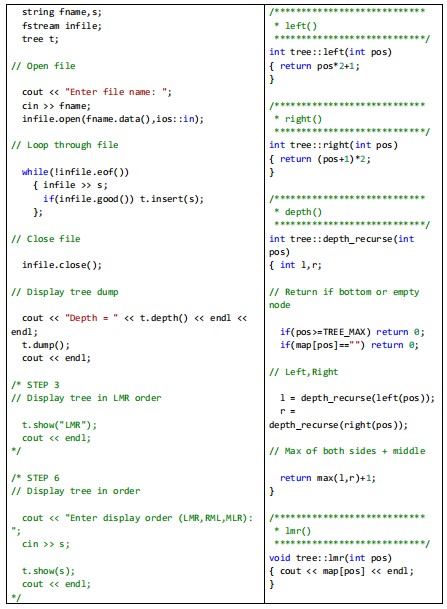
2- Be sure to put the data file in the same directory as the project code files. Run the

program with Data.txt. What is the depth of the tree? What is the index of the last filled

element in the array?

3- Comment out the section in main() that displays the depth and dump of the

tree. Remove the /* */ comments for STEP 3, and run the program again. You should

see just the root of the tree.

4- Modify the tree::lmr() function so that the tree values are displayed in ascending

order. The tree::depth() and tree::depth_recurse() functions may give you

examples for your code.

5- Run the program and save the output.

6- Replace the /* */ comments in main() for STEP 3, and remove the /* */ comments

for STEP 6. Update the tree::show() function, and implement the tree::rml() and

tree::mlr() functions.

7- Run your program with each of the three display orders. Save the output for RML and

MLR.

8- Remove the /* */ comments in main for STEP 8. Implement the tree::find()

function, using the structure of the binary tree.

9- Run the program a few more times to demonstrate that the find function works correctly

(found positions, and not found). Save your output.

Are you struggling to keep up with the demands of your academic journey? Don't worry, we've got your back! Exam Question Bank is your trusted partner in achieving academic excellence for all kind of technical and non-technical subjects.

Our comprehensive range of academic services is designed to cater to students at every level. Whether you're a high school student, a college undergraduate, or pursuing advanced studies, we have the expertise and resources to support you.

To connect with expert and ask your query click here Exam Question Bank