BIOM9660 Sound Processing Assignment

Introduction

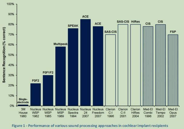
During this course, in the sound processing lecture in week 3 and the introductory sound processing laboratory in week 1, you learnt about different sound processing strategies used in cochlear implants – that is, the translation from a captured sound to electrical impulses delivered via metal electrodes placed within the cochlea. Fig. 1 (adapted from Feng et al. [1]) illustrates the performance differences of the various sound processing strategies in terms of achieving sentence recognition. The single electrode 3M implant of the 1970s/early 1980s was not able to achieve much and required users to extensively lip-read in order to be able to hear and understand speech. When multichannel stimulation came in the 1980s, this brought about a significant change in performance and over time. These strategies have now been improved to the extent that modern strategies such as Advanced Combination Encoder (ACE) can achieve very high performance. The earliest multichannel strategies were the formant-based strategies (F0F2 and F0F1F2). In those strategies, the electrodes closest to formants 1 and 2 were stimulated according to the amplitude of the relevant formant. The stimulation rate was fixed at F0. In subsequent strategies, the features of the sound were reassessed with a focus on finding the most important components of the sound as opposed to its dominating frequencies. This latter approach made the difference between cochlear implants being essentially an aid to lip-reading and finding their place in human achievement as a means of truly “restoring” hearing. Practically speaking, the transition from the formant-based processing strategies to the spectral peak strategies allowed cochlear implant recipients to (among other important things) regularly converse on the telephone.

For those of us who can hear well, it may be useful in relating this to our own experience by considering the challenges of learning a new language. In the early stages of learning, one might expect to detect the occasional word in a new language – akin to the 3M/House single electrode implants of the 1970s. With a bit of practice, some, perhaps several very basic words can be understood or recognised, but the full scope of sentences using these words are only occasionally understood because the missing parts of the sentence have not yet been learned. This is akin to the state of the art in the 1980s with the formantbased strategies, where only a few words were able to be successfully represented in the cochlea using electrical pulses. When the spectral peak approaches came as we entered the 1990s, it was as if overnight the learning phase of the new language was almost over, and suddenly more than 75% of everything became understandable.

Notice that for the past two decades though, the advances have become small and, in some cases, less successful than the preceding strategies. For example, in the device manufactured by Cochlear Ltd, the ACE strategy, adopted in 2002, is still the strategy used today as it gives many people almost 100% speech intelligibility in quiet conditions. There is still significant amount of work to be done though in enabling cochlear implant recipients to hear well in noisy conditions and achieve better pitch perception for hearing music. Perhaps your role in the future will be to deliver that remaining 25% of sound that will make the difference between being able to understand, to being fluent in the language of hearing.

Each of you, through the associated lecture in week 3, the introductory laboratory in week 1 and this assignment, will study and implement into practice, three sound processing strategies: F0F1F2, SPEAK, and CIS to simulate what a cochlear implantee may possibly hear.

Note that the latter two are similar strategies that vary primarily in their presentation rather than processing, but they have a separate history, and are both essential components of modern cochlear implant therapy. If you wish to learn about cochlear implant strategies, one of the best tutorials available freely on the web is one by Dr Philipos Loizou (https://ecs.utdallas.edu/loizou/cimplants/tutorial/). Sadly, Prof Loizou is not living today, but his legacy in cochlear implants will certainly live on!

Expectations

The Assignment is in five parts and constitutes 10% of the total assessment for this course. The first four parts are sub-sections of code, and the final part is the full code along with a 1-page reflection report. All parts are unique and individual MATLAB code must be written by you to implement the sound processing Strategies listed above. The first four parts carry 0.5 marks each and are marked in the labs (these are to help you develop the code in bite sizes). The final submission carries 8 marks which constitutes 5 marks for the full code and 3 marks for the reflection report.

The coding MUST be done using the provided skeleton template. You will have access to Matlab through your university email address. To gain access, all you need to do is create or login to your Mathworks account (http://www.mathworks.com/login) using your UNSW email address and can then access the latest version of Matlab either online (https://matlab.mathworks.com/) or download it onto your computer.

Once logged in to Mathworks, you should also be able to access several Matlab learning courses if you are not familiar with Matlab. You are free to take up any of the available courses, however to be able to complete this assignment, the Matlab Onramp course (2 hours) is compulsory if you have not previously completed it AND if you didn’t attend the first lab where Matlab was introduced to the class. See https://matlabacademy.mathworks.com/ to access the training course. Note, also that there is a plethora of YouTube tutorials for Matlab, several of which will be ultra-helpful to you (particularly ones that teach you how to write functions).

Note on Plagiarism

Students are reminded that plagiarism is absolutely, positively unacceptable and a zero-tolerance approach is taken in this regard in BIOM9660. The MATLAB code components of the BIOM9660 Major Assignment are to be your own work - no exceptions. Other than built-in MATLAB functions, no code from anyone other than yourself is to be submitted. The code and reflection report will be compared with others in the course, previous students in this course as well as online resources including OpenAI tools.

TurnItIn is remarkably good at what it does - that is, finding plagiarised material. If you need to ask whether or not you've plagiarised, you probably already have. Don't do it. If you don't know what it is, find out here: https://student.unsw.edu.au/plagiarism

Sound Files Database

NOTE: Listening to these files before using them in experimentation will compromise the outcome of the group study. There are 280 short sentences - it is STRONGLY RECOMMENDED that you set aside 15 of them at random.

The experimental data from a study by Healy, Yoho et al [2] has been made available for download. The folder “JASA13\data\clean_utterance” contains 280 short speech files. Please select 15 of these files as the sample speech files from which you will generate processed, vocoded speech files for use in your speech perception group experiment. The files contain high quality speech with no background noise.

These "ideal" recordings are much easier to understand than the usual speech + noise that a cochlear implant recipient will experience.

Click http://web.cse.ohio-state.edu/pnl/corpus/Healy-jasa13/YWang.html link to open resource. You must strictly adhere to the coding template available on Moodle. The template provides a skeleton of the six short functions that you must write, a standard test method to test your working code and some standardised output files. Refer to Appendix A in this document for additional information on the code skeleton, installation, testing and submission. Detailed comments should be included in your code in order to guide the marker through what is taking place. If the marker cannot understand the code, the marker cannot provide marks - help yourself by helping them.

The primary aim of your code is to input an original unprocessed sound and using either of three known sound processing strategies (F0F1F2, SPEAK and CIS), process the sound into a vocoded version which will simulate how a sound may be perceived by a cochlear implantee. To achieve this aim, you will need to write six short Matlab functions, the objectives of each of which are as follows:

1. getwav()

In this function, the code must first input one of the sound files from the above-mentioned database (choice up to you but don’t select a file from the 15 you initially selected). The function must then determine the original sampling frequency of the sound and resample if it is not 16 kHz. The tolerance rate for the final sampling rate is set to 10%. This means the final sampling rate must be within 10% of 16 kHz. The resampled sound must then be passed on to the next function.

CODE UP TO HERE CONSTITUTES PART 1 OF THIS ASSIGNMENT, MUST BE WRITTEN BY THE RELEVANT DUE DATE AND SHOWN/MARKED IN CLASS. SEE FIRST PAGE OF THIS DOCUMENT FOR DUE DATES.

2. getFTM()

The objective of this function is to obtain a frequency-time matrix representation of the input sound, formatted into a 2D matrix with:o Electrodes 1-22 making up 22 rows of the matrix, representing frequency in the form of bandpass filters, where 1 is the apical electrode o Epochs 1-x (where x corresponds to the number of epochs) making up the columns of the matrix representing time o F0F1F2: Each cell of the matrix containing the peak amplitude of the epoch in the time domain CIS and SPEAK: Each cell of the matrix containing the peak or average amplitude of the frequency content within a given band-pass filter for a given epoch To achieve this, the sound should first be split into epochs and then each epoch analysed.

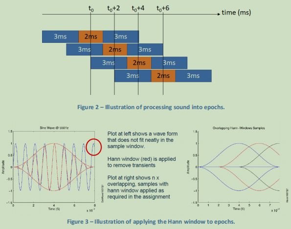
The epoching process will be slightly different from the one done in the introductory lab of week 1 so careful attention must be paid. Each epoch must be 8 ms (128 samples) long with its centre point shifted by 2 ms from the previous epoch (therefore each epoch will overlap the previous epoch by 6 ms, 3 ms before and 3 ms after the centre point). See Fig.2 below for an illustration showing how to create overlapping epochs.

Thus, the key difference to the lab is that here, epochs will be overlapping whereas in the week 1 lab, you will have created non-overlapping epochs. Each created epoch must also be smoothed using a Hann function https://en.wikipedia.org/wiki/Hann_function. The purpose of the Hann function is so that abrupt epoch edges do not create unnecessary edges (high frequency content) in your processed sound.

See Fig.3 for an illustration on how Hann windowing works and how the overlapping smoothed epochs may look.

Each smoothed epoch is to be then further processed according to the three sound processing strategies.

This part of the code will find the frequency content of each epoch either through finding formants or through fourier transform.

F0F1F2:

For the F0F1F2 strategy, epochs can be processed for frequency analysis using the linear prediction coefficients that you made use of in the week 1 lab. Once you determine the first two formants (F1 and F2) in each epoch, you must assign an appropriate amplitude value to the appropriate electrodes in the FTM, based on the formant frequency values in the epoch and the frequency range of each electrode. To know what frequency range corresponds to each of the 22 electrodes, use the function “getBandInfo()” that has been written for you. When you call upon this function, it will return a 22x4 matrix where each row represents an electrode. Column 1 of this matrix has the centre frequency of the band, column 2 has the lower cutoff frequency, column 3 has the higher cutoff frequency and column 4 has the width of the band. The higher and lower cutoff frequency information should help you determine which electrode to stimulate for a particular formant. With regards to the amplitude assigned for the two formants, simply use the time domain signal of the epoch and calculate the peak of that signal. For the unused electrodes in each epoch, set the FTM value to zero. Therefore, the FTM for the F0F1F2 strategy will essentially have 22 rows, number of columns equalling the number of epochs and each column containing only two nonzero values. Note, all this time we have been using the name F0F1F2, but we know F0 represents the rate of stimulation in cochlear implants and therefore is not relevant to the FTM, so we could have essentially called this strategy the F1F2 strategy

CODE UP TO HERE CONSTITUTES PART 2 OF THIS ASSIGNMENT, MUST BE WRITTEN BY THE RELEVANT DUE DATE AND SHOWN/MARKED IN CLASS. SEE FIRST PAGE OF THIS DOCUMENT FOR DUE DATES.

CIS and SPEAK:

For the SPEAK and CIS strategies, processing is much simpler. Once you form the epochs and smooth them with the Hann function, you will need to use the fast fourier transform (FFT) to analyse frequency content in each epoch. For each epoch, the FFT output will be 128 samples long since each epoch is already that length (see above section on epoch creation). To combine the FFT output into the frequency bands simply call upon the function “combineBands(data)” where ‘data’ represents your FFT output variable.

Once you have analysed all epochs for all strategies, the end result will be your final FTM which will be passed on to the next function.

3. process()

The objective of this function is to further process the FTM values and only choose the ones of interest. In the case of the F0F1F2 strategy, in each epoch you will have assigned two electrodes to non-zero values (peak amplitude of the signal in that epoch). In the case of the CIS strategy, all 22 electrodes will have FTM values. In the SPEAK strategy, electrodes with the largest 8 FTM values will be used. The first step in the ‘process’ function (for all three strategies) will be to normalise the FTM from zero to one, this can be done by dividing every element of the FTM by the maximum of the whole FTM. Then, as a second step, for the SPEAK strategy only, you should choose electrodes with the largest 8 values for each epoch and set the remaining electrodes to zero. You can now pass the processed FTMs to the next function.

CODE UP TO HERE CONSTITUTES PART 3 OF THIS ASSIGNMENT, MUST BE WRITTEN BY THE RELEVANT DUE DATE AND SHOWN/MARKED IN CLASS. SEE FIRST PAGE OF THIS DOCUMENT FOR DUE DATES.

4. applyDR()

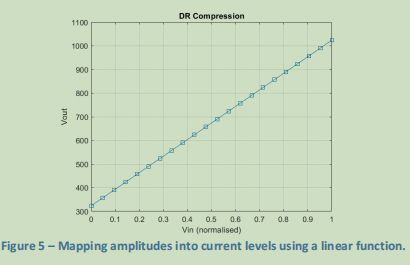
The FTM should then be further processed using a dynamic range procedure, where the outputs of sound processing are converted to current levels that will be used for each electrode. The stimulus amplitude range will be 324-1024 microamps for all strategies. Note that an output of zero from the FTM will receive zero current. The maximum output in the FTM (AMAX which should be equal to 1 provided you normalised the FTM) should be re-assigned to 1024 microamps (also called the C level). The ‘T’ level will be the lowest (AMIN) non-zero output in the FTM and should be re-assigned to 324 microamps. In this manner, the useful dynamic range will be limited to 10 dB - that is, the difference between the T and C levels will represent a 10 dB dynamic range. You are free to use a linear function or logarithmic function to choose the values in between AMAX and AMIN. See Fig. 5 which applies a linear function.

CODE UP TO HERE CONSTITUTES PART 4 OF THIS ASSIGNMENT, MUST BE WRITTEN BY THE RELEVANT DUE DATE AND SHOWN/MARKED IN CLASS. SEE FIRST PAGE OF THIS DOCUMENT FOR DUE DATES.

5. plotSignal()

This is a simple function to plot the original sound you have chosen to process in the time domain. Ensure that you label both your axes and plot appropriately as labels also carry marks!

6. plotElectrodogram()

This function will plot the FTM into a heat map with electrodes on the y-axis and time on the x-axis. The apical electrode must be located on the top of the plot. Ensure that you label both your axes and plot appropriately as labels also carry marks! For this plot, you will also need a legend for the z-axis (i.e. the colour map).

CODE UP TO HERE CONSTITUTES THE FINAL CODE, MUST BE WRITTEN BY THE RELEVANT DUE DATE AND SUBMITTED IN MOODLE AS A MATLAB “.m” FILE. SEE FIRST PAGE OF THIS DOCUMENT FOR DUE DATES.

YOU MUST USE THE “classCochlear.m” SKELETON FILE TO WRITE YOUR FUNCTIONS IN THE SPACE PROVIDED. ONCE YOU HAVE WRITTEN ANY PART, RUN THE CODE USING THE “cochlearProc.m” file. See APPENDIX FOR DETAILS ON HOW TO RUN AND TEST YOUR CODE.

Are you struggling to keep up with the demands of your academic journey? Don't worry, we've got your back! Exam Question Bank is your trusted partner in achieving academic excellence for all kind of technical and non-technical subjects.

Our comprehensive range of academic services is designed to cater to students at every level. Whether you're a high school student, a college undergraduate, or pursuing advanced studies, we have the expertise and resources to support you.

To connect with expert and ask your query click here Exam Question Bank