The Capital Investment Analysis Application of Activity-Based Costing Techniques in the EDUC Electric Distribution Utility Company

1. INTRODUCTION

Activity Based Costing is one of the tools and techniques that was covered in the CMA program, and I will demonstrate that it is very useful in providing decision-oriented information to senior management in my organisation that will ultimately enhance its corporate value.

The company that is the focus of my study is the EDUC Electric Distribution Utility Company, which serves around 25 percent of the Indian population.

I worked as one of the Financial Controllers of EDUC.

1. THEORETICAL FRAMEWORK

Traditional investment is based on the cash flow impact of each alternative, a process that does not take into account non-monetary decision parameters such as quality and efficiency (Angelis & Lee, 1996). It compares investments proposed by department managers based on the benefits to each department, without analysing the effect of the investment on the activities and strategic goals of the company.

This framework has been applied in EDUC which serves around 25 percent of the Indian population. Its capital expenditure in 2005 is worth around three percent compared to its total assets.

Activity-Based Costing (ABC) is a methodology that measures the cost and performance of activities, resources and cost objects (Miller, 1996).

The resources are classified as: capital expenditures (CAPEX) and operating expenses. For CAPEX, the cost elements are labor, transportation, contracted services and other expenses. Materials are excluded in the CAPEX to highlight the cost of performing the activities.

There are two axes to the ABC model (Fig. 1) as developed by the Consortium for Advanced Manufacturing International (CAM-I). The vertical one deals with the cost assignment view. The resource contains all means upon which the selected activity can draw. The resource cost assignment process contains the structure and tools to attribute costs to the activity. The activity is where work is performed. The activity cost assignment process contains the tools to assign costs to cost objects, utilizing activity drivers as the mechanism to accomplish this assignment (Miller, 1996).

The horizontal axis contains the process view. The cost driver is the agent that causes the activity to utilise resources to accomplish some designated work. In this view the activity is some type of active work centre. The performance measure of activities entity houses the evaluative criteria by which the organisation can determine the efficiency and effectiveness of the activities work effort (Miller, 1996).

• ACTIVITY-BASED INVESTMENT DECISION ANALYSIS FRAMEWORK

Phase I. Project Analysis Method

Investment decisions are anchored on net present value (NPV) method, internal rate of return (IRR) method and others. The net present value criterion is the most widely accepted decision rule in academia (Sick, 1997).

In the project analysis method, the NPV and IRR methods will be used in the formulation of investment decisions. ABC data will be used in the cash flow variables such as initial investment and operating and maintenance expenses.

Phase II. Project Prioritisation Method

The project prioritisation method in Fig. 2, is a tool for systematic selection among various alternatives with several criteria. It consists of three basic selection methods: cost impact; performance impact; and quadrant analysis.

This presents the application of the analytic hierarchy process as a tool. The attributes are represented by a two- tiered cost impact model and a three-tiered performance impact model. Table I presents the methodology.

Analytic Hierarchy Process (AHP) was developed to structure complex, multi-attribute problems. It creates a hierarchical structure based on goals, criteria, sub-criteria and alternatives (Angelis & Lee, 1996; Saaty, 1982).

Formulating the problem (Fig. 3) is the first step. The top level is the objective. Subsequent levels are constructed so that elements within a level are the same order of magnitude, as they are compared to each other in relation to elements of the next higher order. The levels below the overall objective are referred to as attributes and sub-attributes and consist of the decision criteria. The first level of attributes is the strategic goals. Below are activities as the sub- attributes. At the lowest level are the decision alternatives (Angelis & Lee, 1996; Zahedi, 1986).

The decision maker determines the importance of each element in a level. This is done by pairwise comparisons of the elements at a given level relative to each of the criteria at the next higher level. Then, calculate the overall rating of each alternative by multiplying the weights along each path of the hierarchy leading to an alternative, and then adding these products for each decision alternative.

Cost Impact

Figure 4 illustrates the cost impact model of the new method. By analysing the resources consumed as a company performs its activities and measures its performance, management can identify areas where change may achieve significant cost reductions (Angelis & Lee, 1996).

Performance Impact

Figure 5 illustrates the performance impact model of the new method. Performance measures allow management to influence activities that are critical to strategic goals. Activities provide a tangible link between indices and objectives. Without this link, management is left with intangible benefits from long-term goals that they perceive as important but unmeasurable (Angelis & Lee).

Quadrant Analysis

Combine the results of the cost and performance models to select the best investment. The models assign a weighted evaluation to each investment alternative, one for cost and one for performance (Angelis & Lee, 1996). Use a graph in Fig. 6 to select the best alternative. Investments falling in quadrant III are the most preferred, while those falling in quadrant II would be the least preferred (Angelis & Lee, 1996).

1. METHODOLOGY

The ABC&M office of the company initiated the Activity-Based Management project with focus on ABC information. One such application is strategic investment planning decisions. Thus, the capital investment decision was developed based on the principles of capital budgeting and capital rationing.

A. Project Simulation Methodology

The concept was simulated in a pilot application. Project teams were formed to help in the proof of concept stage. There was a meeting after the concept presentation to the steering committee with the heads of the following offices: Planning; Substation; Distribution and Subtransmission. The electric capital projects were classified into: substation; sub-transmission line; and distribution line projects.

For the project analysis method, the steering committee members agreed to analyse two projects for each category. The mandate was to determine: the activities of the initial investment cash out flow variable; the activities of the operations and maintenance cash outflow variable; the financial viability of each project.

For the project prioritisation method, the steering committee agreed to subject 23 projects for implementation to undergo the new method and compare the results with the existing method. They agreed to use the proposed method with modifications subject to the availability of data. The modifications were: the non-inclusion of the activities; and cost savings will be derived from the benefits of the projects.

B. Project Analysis Method

A workshop was held. Sample projects similar to Tables II, III, & IV, were made available to the participants and they were guided on how to use ABC data.

Aside from direct costs, ABC resources also include non-electric asset costs and shared services costs. Asset costs are incurred in the use of company assets, to perform the activities. They come in the form of depreciation, property taxes, insurance, interest expenses and amortisation on debt expenses. Shared services costs are incurred and passed on by another internal organisation in providing support to other organisations. The reassignment is from the performing organisation to the benefiting organisation, then to the benefiting organisations activities.

Cash flow variables were identified as investment cost; operation and maintenance expense and overhead expense variables. The ABC data in this method does not include depreciation expenses of asset costs.

For the investment cost, the existing practice utilises the amount in the work order system. The method offers theactivity cost data of the planning, design and construction activities to replace the labour, transportation, contracted services and storage costs. The direct material costs from the system will remain part of the method. The activity cost data shall be derived from the previous years ABC information.

The challenge in the investment cost is the identification of CAPEX activities related to a particular type of project like substation, subtransmission lines and distribution lines, and identify the number of times an activity will be used. The activity driver should: correlate with the consumption of the activity; encourage improved performance; and already be available and/or have a low cost of collection (Miller, 1996).

A second workshop was held to analyse the Activity-to-Project Maps each team prepared. This map is a list of activities of a particular type of project. Each project has two maps, one for the initial investment and the other is for the operations and maintenance.

The initial investment using ABC information (Table III) is made up of capitalised activity costs for a particular type of

project. In this case, the project is an Upgrading of a 115Kilovolt Subtransmission Line.

For Table IV, it is important to classify the activities into value-adding and non-value adding. If possible, include only the value-adding costs as part of the relevant expenses.

C. Project Prioritisation Method

The steering committee agreed to subject all 23 projects to the new method and compare them with the existing method. They divided the projects into: Substation; Subtransmission; and Distribution Lines. They agreed that the main criteria for the analytic hierarchy process (AHP) should be tied up to the goals of the Company. The AHP main criteria are: Adequacy refers to the capacity to accommodate new loads; System Reliability and Flexibility refers to the ability to minimise power interruptions; Public Safety refers to the reduction of hazards; System Loss refers to the ability to reduce technical system loss; and Power Quality refers to the improvement in the supply of electric power to sensitive customers.

The discussion was centred on the new method especially on the use of analytic hierarchy process. One main concern raised during the discussions is the guideline on AHP which states that no more than nine elements in any cluster. The original method on the performance impact model requires the use of AHP on the alternatives. In a utility company, the number of alternatives may surpass the limit of nine projects.

The issue on the limitations of nine projects was resolved. Instead of AHP on the last level, the revised performance impact model requires the performance values of each project with respect to the performance driver.

Fig. 7 shows the weights of the main criteria in the pairwise comparison performed by the project team members.

Cost Impact Model

The initial application of the model started with the identification of the main criteria. The projects are then placed after the main criteria (Fig. 8). The main objective in pursuing this modified model is to sell the concept to prospective customers without the intricacies involved in the gathering of ABC information. The cost savings information did not come from the savings on resources consumed by activities. Cost savings were replaced by cost benefits with the use of the existing financial analysis. Once the prospective users agree that the concept improves their existing method, ABC information build-up will be the next logical step to pursue the complete ideal model in the theoretical framework.

Performance Impact Model

Figure 9 is the initial application of the model in the project simulation. Notice that the activities are not included. The model introduces the performance measures as sub-criteria. These are linked to the main criteria using the analytic hierarchy process. This model incorporates the performance of each project with respect to the performance driver of each main criterion contributing to it. There are no limits in the number of alternatives for as long as performance measures are defined.

Comparative Results Between the Net Present Value and Project Prioritisation Method

In the new method, the ranking is based on shortest distance to the coordinate (1,1) in the cost savings versus performance graph (Fig. 6).

Tables V, VI and VII show the comparison between the results of Project Prioritisation Method and NPV.

1. CONCLUSIONS AND RECOMMENDATIONS

A. Project Analysis Method

There were realisations that most activity drivers did not represent realistic consumption of the activities and most activity drivers and costs did not have accurate data because of the poor utilisation of the work order systems by the construction, maintenance and operations personnel.

The project teams decided to suspend the implementation of the proposed method pending the resolution of the following recommendations: determine the possibility of using the work order systems to generate the driver data; and develop a method to forecast the operation and maintenance activities given the 30-year economic life span of projects.

B. Project Prioritisation Method

The models are flexible enough to adapt to the present limitations of available information.

This method can be used in various decision analyses such as: to buy or to lease; to outsource or to hire; business development applications; new product development; performance ratings and other similar applications.

REFERENCES

Angelis, D. I. and Lee, C. Y. (1996) Strategic Investment Analysis Using Activity Based Costing Concepts and Analytic Hierarchy Process Techniques. International Journal for Production Research, Vol. 34, No. 5, 1331-1345.

Miller, J. A. (1996), Implementing Activity-Based Management in Daily Operations, New York, John Wiley & Sons, Inc.

Saaty, T. L. (1982), Decision Making for Leaders, Lifetime Learning Publications, California. Sick, G. (1997), Investment Decision Analysis, University of Calgary Press, Calgary.

Zahedi, F. (1986), The Analytic Hierarchy Process A Survey of the Method and its Applications, Interfaces Vol. 16, No. 4, pp. 96-108.

SUMMARY OF FIGURES AND TABLES

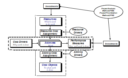
Fig. 1. CAM-I Cross with Investment Impacts

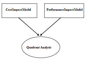
Fig. 2. Project Prioritisation Method

TABLE I

INPUT PROCESS - OUTPUT FRAMEWORK

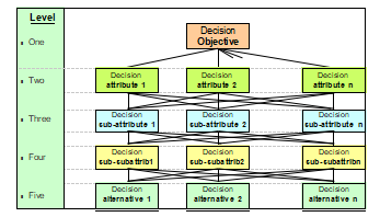
Fig. 3. Analytic Hierarchy Process Model

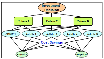
Fig 4. Cost Impact Model

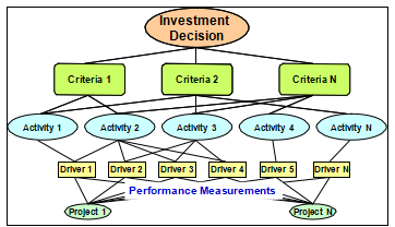
Fig. 5. Performance Impact Model

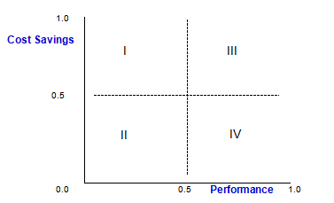
Fig. 6. Cost Savings vs. Performance

TABLE II COMPARATIVE CASH FLOW VALUES

TABLE III

INITIAL INVESTMENT

TABLE IV OPERATIONS & MAINTENANCE

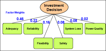
Fig. 7. Main Criteria

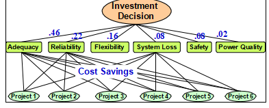
Fig. 8. Cost Impact Model Initial Application

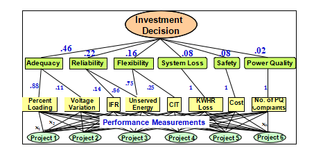
Fig. 9. Performance Impact Model Initial Application

TABLE V SUBSTATION PROJECTS

TABLE VI SUBTRANSMISSION LINE PROJECTS

TABLE VII DISTRIBUTION LINE PROJECTS