CMP9783M Neural Computing Assessment

Section 1 LIF neuron model with adaptation (50%)

Neuroscience goal: Understand the reciprocal impacts of adaptation currents on spike trains and spike trains on adaptation currents; understand how limits on the firing rate and mean membrane potential depend on the spiking mechanism.

Computational goal: Simulate coupled differential equations with two variables; analyze simulation results and plot appropriate features of the simulation, for example, depending on the number of spikes produced.

In this exercise, you will analyse the impact of adaptation currents on the f-I curve of a neuron.

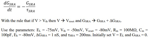
1. Write code to simulate the LIF model with an adaptation current so that the full model becomes:

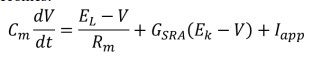
and

a. Simulate the mode neuron for 1.5s, with a current pulse of Iapp = 500 pA applied from 0.5 s until 1.0 s. Plot your results in a graph, using three subplots with the current as a function of time, the membrane potential as a function of time and the adaptation conductance as a function of time stacked on top of each other. (10 points)

b. Now simulate the model for 5 s with a range of 20 different levels of constant applied current such that the steady state firing rate of the cell varies from zero to 50Hz. For each applied current calculate the first interspike interval and the steady-state interspike interval. On a graph, plot the inverse of the steady-state interspike interval against applied current to produce an f-I curve. On the same graph plot as individual points (e.g. as crosses or squares) the inverse of the initial interspike interval. Comment on your results. (10 points)

2. Write a code to simulate the Adaptive Exponential Leaky Integrate-and-Fire (AELIF) neuron

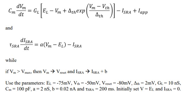
a. Simulate the model neuron for 1.5 s, with a current pulse of Iapp = 500 pA applied from 0.5 s until 1.0 s. Plot your results in a graph, using two subplots with the current as a function of time plotted above the membrane potential as a function of time. (10 points)

b. Now simulate the model for 5 s with a range of 20 different levels of constant applied current such that the steady state firing rate of the cell varies from zero to 50Hz. For each applied current calculate the first interspike interval and the steady-state interspike interval. On a graph plot the inverse of the steady-stateinterspike interval against applied current to produce an f-I curve. On the same graph plot as individual points (e.g. as crosses or squares) the inverse of the initial interspike interval. Comment on your results. (10 points)

Section 2 Hodgkin-Huxley model as an oscillator (50%)

Neuroscience goal: Gain appreciation of the Type-II properties of the Hodgkin-Huxley model.

Computational goal: Careful transposition of mathematical formulae and parameters into computer code; practice of simulations with several interdependent variables.

In this exercise, you will simulate a full four-variable model similar to the original HodgkinHuxley model (though using modern units). The four variables, sodium activation, m, sodium inactivation, h, potassium activation, n, and membrane potential, V, will all be updated on each timestep, since they depend on each other. Initial conditions should be 0 for all gating variables, and EL for the membrane potential, unless otherwise stated

1. Set up a simulation of 0.35 sec duration of the Hodgkin-Huxley model as follows:

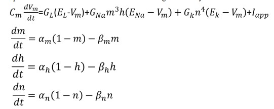
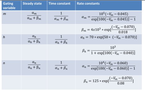
where the parameters are given in table 1 and the rate of constants are the instantaneous functions of membrane potential given in table 2.

Table 1. Parameter values for HH model

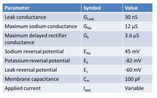
Table 2. Gating variables of the HH model

Initially set the applied current to zero and check the membrane potential stabilizes at -70.2mV. (5 points)

2. Produce a vector for the applied current that has a baseline of zero and steps up to 0.22 nA for a duration of 100 ms beginning at a time of 100 ms. Plot the applied current on an upper graph and the membrane potentials response on a lower graph of the same figure. (you should see subthreshold oscillations, but no spikes). (5 points)

3. Alter your code so that the applied current is a series of 10 pulses, each of 5 ms duration and 0.22 nA amplitude. Create a parameter that defines the delay from the onset of one pulse to the onset of the next pulse. Adjust the delay from a minimum of 5 ms up to 25 ms and plot the applied current and membrane potential as in question 2 for two or three examples of pulse separations that can generate spikes. Be careful (especially if using the Euler method) to repeat your simulation with your time step reduced by a factor of 10 to ensure you see no change in the response, as a sign you have sufficient accuracy in the simulation. (A timestep of as low as 0.02 ?s may be necessary.). Describe and explain your findings. (10 points)

4. Now set the baseline current to be 0.6 nA. Set the initial conditions as Vm(0) = -0.065V, m(0) = 0.05, h(0) = 0.5, n(0) = 0.35. (Note that the 0 in parenthesis indicates a time of t = 0, which corresponds to element number 1 in an array.) Apply a series of 10 inhibitory pulses to bring the applied current to zero for a duration of 5 ms, with pulse onsets 20 ms apart. Plot the applied current and the membrane potentials response as in questions 2 and 3. Describe and explain what you observe. (10 points)

5. Now set the baseline current to 0.65 nA. Set the initial conditions as Vm(0) = -0.065 V, m(0) = 0.05, h(0) = 0.5, n(0) = 0.35. Increase the excitatory current to 1 nA for a 5 ms pulse at the time point of 100 ms. Plot the applied current and resulting behavior in the same manner as in questions 2, 3, and 4. Describe what occurs and explain your observation. (10 points)

6. Repeat 5 with the baseline current of 0.7 nA, but set the initial conditions as Vm(0) = - 0.065V, m(0) = 0, h(0) = 0, n(0) = 0. As in question 5, increase the excitatory current to 1 nA for a 5 ms pulse at the time point of 100 ms. Plot the applied current and resulting behavior in the same manner as in questions 2-5. Describe what occurs and explain your observation, in particular by comparing with your results in question 5. (10 points)

Are you struggling to keep up with the demands of your academic journey? Don't worry, we've got your back! Exam Question Bank is your trusted partner in achieving academic excellence for all kind of technical and non-technical subjects.Our comprehensive range of academic services is designed to cater to students at every level. Whether you're a high school student, a college undergraduate, or pursuing advanced studies, we have the expertise and resources to support you.

To connect with expert and ask your query click here Exam Question Bank